Calculating Demand
The purpose of calculating demand is to establish a baseline for forecasting future demand. Whereas data on workforce supply is typically in plentiful supply within an organisation, data on demand is often scant and fragmented. This delta, and the complexity of the subject, is why we conduct a baselining activity as part of the demand stage rather than as part of the baseline stage. If we are operating at a macro level, there would be little disadvantage to conducting this exercise earlier. At a meso and micro level, we risk the economy of our effort by collecting and analysing too much demand data before we understand fully the nature of the workforce supply who will be servicing that demand.
Last month’s web page on the workforce performance model gave us a clear framework that a greater level of resource is required than is indicated by volumes and processes when we convert from contract time to productive time. The product of labour is based on the productivity of a single worker, not the productivity of the productive time of a single worker. This provides us with two approaches that are output-based or input-based.
An Output-Based Approach
This approach seeks to identify the relationship between the workforce and the outputs they produce, which are known as products of labour and illustrated in the following diagram

The average product of labour (APL) is the average individual output for the workforce. For 10 workers producing 100 units, the APL is 10. The APL increases at a slow rate as the organisation benefits from the advantages of additional workers. These economies of scale reach a peak and then become diseconomies of scale as average output improves. The 10 workers with an APL of 10 may operate a production line where increasing hands allow the average output to increase. When that team reaches maximum capacity for space, and workers start bumping into each other on the production line, the APL starts to reduce. Whereas APL is the average, MPL is the marginal product of labour: the change in output from adding an additional worker. Initially, there are increasing marginal returns, the benefit of adding a worker is greater than the benefit of adding the previous worker. This quickly hits a peak before descending into diminishing marginal returns where each additional worker continues to increase the overall output but made less of a difference than the last. There are two key factors in play at this point: communication and divisibility.
- As more workers are added to the process, there is a polynomial growth in lines of communication as more people need to pass information to each other. This combinatorial explosion in demand erodes the benefit created by the marginal return.
- The second factor, divisibility, is that some activities are not easily divided and so the addition of workers does not add the same benefit as the initial workforce. At the end of the MPL curve, we hit the worst case, diminishing returns, where the organisation is saturated and the addition of an extra worker results in a decrease in output. This is the point, perhaps, where the organisation reaches the Malthusian catastrophe of having too many workers for the number of machines or space they have, and work suffers as a result.
Aligning high-level output data with worker levels will allow us to map a number of points on both the APL and MPL curves to understand current levels of derived demand for workers and how that varies.
The benefits of this approach are that the data on outputs is often the most readily available and is much easier to calculate. The limitations of this approach are that it does not connect with input data and is less useful at meso and micro levels of the organisation.
An Input-Based Approach
The input-based approach calculates the relationship between inputs, workers and outputs. It is the most comprehensive approach to calculating demand. To do this, we need to first understand the input volumes and how those volumes translate into the derived demand for labour.
Determining Input Volumes The start point for determining input volumes is through the analysis of time series data; a collection of sequential data points over a time period. The source of this time series data will sit within our supply chain and be different depending on the nature of our organisation. In a best-case, the organisation will also have data around their business operations including the flow of demand in and around the business. It is more likely, however, that we will be looking at whatever data is available. Those producing goods will have data on their inbound logistics of primary or secondary sector products; equally, there will be data on the outbound logistics of the final products going to market. Other types of organisation, such as those providing a shared resource, would have data on their customers and their usage rates. The level of the organisation and the planning horizons will dictate the nature of this data. Creating a calculation for a short planning horizon at a micro level can necessitate minute by minute breakdowns of demand data, planning at higher levels and longer timeframes can be achieved through aggregated datasets. Analyses of the trends in this data will show not only both the initial inputs and final outputs, but also the associated inputs and outputs throughout the entire internal supply chain.
Establishing Derived Demand for Labour
A Top-Down Method
As process systems and controls will typically remain a constant, it is the analysis of the trends in inputs, outputs and resources that will indicate the derived demand for labour. Regression analysis of those trends will indicate the causal relationship between the process steps to give an indication of the ratio of inputs and outputs in relation to the workforce.
A Bottom-Up Method
In the absence of clear top-down information, or when planning at either a micro level or in horizon one, we may require a bottom-up approach to calculate our demand. The basis of this will require a work-study to understand the nature of the process. At the lowest level, this will necessitate a time and motion (T&M) study, a timed review of each process step to understand the expected duration of each process step at a micro level. At a higher level, an average handling time (AHT) may be more appropriate; this is the time for an overall process rather than a detailed time and motion study of each specific process step. At the next level, we may look at individual workers or teams; for this group, the day in the life of (DiLo) may be the best approach. DiLo can be particularly useful when quantifying the activity of knowledge workers who may follow irregular processes. A DiLo is an indication over a single day (or the average of a number of days) to list the types of work and interactions and the time spent on these.
T&M, AHT and DiLo are all effective bottoms up methods for establishing derived demand based on current work. It may be the case that we are looking to calculate based on new types of work, for example a new service offering, or new ways of working following a process change. For this, looking at benchmarks can be an immensely helpful guide. Either within our own organisation or across the industry in other organisations, there will be benchmarks that could be detailed or abstract.
Calculating the Labour Requirement
Establishing the labour requirement, the target level of FTE, is based entirely on the workforce performance model shared last month .

We first start with the input volume levels, the quantity of input, and the processing time, how long it takes to convert that input into outputs, to establish the Productive Time

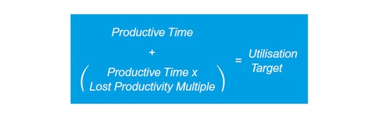
The next step in calculating the labour requirement is to add to Productive Time a Lost Productivity multiple, which comprises the speed to competence and the levels of underperformance. Speed to competence is the time it takes for a new starter to become fully productive as a result of their training; underperformance are those existing workers who are not delivering at the productive level. This creates a utilisation target.

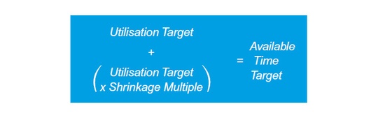
A shrinkage multiple, based on the percentages of FTE and headcount shrinkage, are added to the utilisation target to create an available time target. For example, if the overall impact of shrinkage on a single FTE is 8 hours, or 0.2 FTE, the multiple is 0.25)
Next, we add a core absence multiple to available time to create the target time. The core absence multiple is based on holiday levels. If we take a standard offering within the United Kingdom of 8 public holidays and 25 days of holiday entitlement, the multiple is 0.145.